Types of statistical methods: statistical inference
Descriptive statistic >> Statistical inference > Value of interval estimates | Nonparametric methods
What we take most pride in is our inference, never devoid of error probability! But fear scared – error probability is usually negligible.

Dembitskyi S. Types of statistical methods: statistical inference [Electronic resource]. - Access mode: http://www.soc-research.info/quantitative_eng/7.html
As we mentioned earlier, statistical inferences are used to project the data from the sample to the entire population. Random errors typical of sampling may lead to the fact that the sample will not be an [accurate enough] model of the population. In fact, the sample is never a 100% accurate model of the population, but only its more or less distorted variant. In order to estimate these distortions and, therefore, to make more accurate conclusions about the population statistical inferences are used.
First of all, they allow us to estimate the probability that the determined relations, differences, values, etc. are characteristic only of the sample, but not of the population. The logic here is as follows: if the probability is high, it is stated that the sample parameters are not typical of the population, and vice versa – if the probability is low, it is assumed that the respective sample parameters indicate the population parameters.
First of all, they allow us to estimate the probability that the determined relations, differences, values, etc. are characteristic only of the sample, but not of the population. The logic here is as follows: if the probability is high, it is stated that the sample parameters are not typical of the population, and vice versa – if the probability is low, it is assumed that the respective sample parameters indicate the population parameters.
It is important to remember that achieving a 100% guarantee that the results obtained in the study are characteristic of the population is only possible when the sequential research is conducted, i.e., the survey includes all representatives of the population. But this is no longer a sampling study and does not involve statistical inference.
In its most general form, statistical inference can be divided into two groups: 1) interval estimation (calculating the interval where the mean or proportion of the population must occur with a given probability); 2) statistical hypothesis testing (probabilistic inference about certain sample parameters reflecting (or not) the parameters of the population).
To view each groups, click on one of the buttons below.


Interval estimation
In many cases it may be necessary to estimate the corresponding parameter of the population on the basis of a single sample parameter (its mean or proportion). If the sample is large enough (over 100 observations), it is possible to calculate the interval where the true value will occur with a given probability, with the help of the properties of the normal distribution curve, as well as the central limit theorem.
As you may recall from Chapter II, the distribution of sample means is normal. Consequently, the probability of obtaining a sample with the mean close enough to the population mean is rather high. However, even when the sample mean is essentially different from the population mean, the confidence interval [in most cases] will include the true value. Only in very rare cases we may obtain the sample where the sample and population parameters are so different that the true value will not occur in the confidence interval.
We will not go into detail of the relevant evidence and examples, but will discuss the technique of calculating confidence intervals.
Confidence intervals for the means
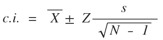
where Z is the standardized value determined by the alpha level or p-value (the probability that the true value will not occur in the confidence interval);
s – standard deviation for the sample;
n – sample size.
It is obvious that s and n are known from the study itself. In its turn, Z is determined using the chart of standardized values:
s – standard deviation for the sample;
n – sample size.
It is obvious that s and n are known from the study itself. In its turn, Z is determined using the chart of standardized values:
Confidence level |
Alpha (р) |
Z-value |
90% |
0,10 |
±1,65 |
95% |
0,05 |
±1,96 |
99% |
0,01 |
±2,58 |
99,9% |
0,001 |
±3,29 |
Confidence level indicates the probability of the true value occurring in the interval calculated.
Here is an example. Let us assume the sample (n = 300) tells us that the mean for monthly income for the citizens of Kiev is 4000 UAH, and the standard deviation is 75 UAH. If we are satisfied by the error probability of 5% (alpha – 0.05), then Z = ± 1,96.
Here is an example. Let us assume the sample (n = 300) tells us that the mean for monthly income for the citizens of Kiev is 4000 UAH, and the standard deviation is 75 UAH. If we are satisfied by the error probability of 5% (alpha – 0.05), then Z = ± 1,96.
Hence:
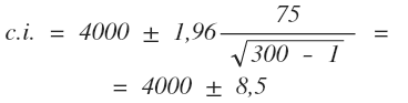
Thus, the true value for the citizens of Kiev must occur in the interval between 3991.5 UAH and 4008.5 UAH with 95% probability.
Confidence intervals for proportions
Confidence intervals for proportions
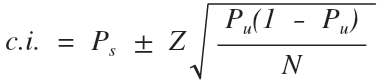
As compared with the previous one, this formula also includes sample size and Z-value. The latter is also determined using the chart above.
Other components include:
Ps – proportion value for the sample;
Pu – proportion value for the population.
The most attentive of you might wonder where to look for Pu if we want to use Ps for its estimation. Or if we know Pu, then why do we need Ps? Indeed, we only need Ps to estimate the unknown Pu. The way out of this situation is quite simple – we assume that Pu is the value (as you remember, for proportions it can vary from 0 to 1) that would give us the highest value of the expression of Pu (1-Pu). Then the confidence interval itself will have the highest value (all other conditions being equal / ceteris paribus). In fact, the researcher must deliberately increase the interval, since a longer interval is more likely to include the true value for the population we are trying to determine. This value is 0.5: 0.5 (1-0.5) = 0.5 * 0.5 = 0.25
Now here is an example. Let us assume that according to the results of the pre-election survey, 17% of the population are ready to vote for the oppositional party (Ps = 0,17), the sample size is 1,200 people, and the alpha level is 0.01.
Then:
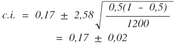
Consequently, from 15% to 19% of the population will vote for the oppositional party with 99% probability.
- default_titleХили Дж. Статистика. Социологические и маркетинговые исследования. - К.: ООО "ДиаСофтЮП"; СПб.: Питер, 2005. - 638 с.
- default_titleМалхотра Н. Маркетинговые исследования. - М: Вильямс, 2007. - 1200 с.
- default_titleField A. Discovering statistics using SPSS. - London, Thousand Oaks, New Delhi: Sage, 2009. - 822 p.
- Show More
Statistical hypothesis testing
With statistical hypothesis testing, based on the data obtained, the researcher verifies the hypothesis stating that all determined relations between phenomena or differences between groups are the result of random errors.
Statistical hypothesis testing consists of the following steps: 1) Verifying assumptions. 2) Formulating statistical hypotheses. 3) Determining alpha level (p-value). 4) Calculating empirical test value and degrees of freedom. 5) Applying theoretical distribution: defining critical value and its comparison with empirical value.
Let us illustrate the basis of statistical hypothesis testing with the chi-square test for independence. This test determines whether there is a relationship between two variables, based on contingency tables. It is a nonparametric test, i.e. it does not require verifying assumptions about the form of distribution of sample statistics.
Step 1. To use the chi-square test, the data must meet only two assumptions:
a) Independent random samples are used. Independent samples occur when respondent selection for one sample does not affect respondent selection of another sample.
First, these data must be obtained from randomly selected students (for example, with the random selection from the list of all university students). In this case, the sample will also be independent – any male or female not yet in the sample can be further selected, no matter who was selected last.
b) Variables belong to a nominal scale. Since nominal scales are considered the "weakest", the use of ordinal and metric variables is also possible (after the number of their categories is reduced to the necessary amount).
For example, look at the table below, where the influence of students’ gender on their learning efficiency is tested:
Green represents the marginal frequencies in lines and columns. They will be needed later to calculate the expected frequencies.
| Efficiency | Gender |
Total
|
|
Female |
Male |
||
| Satisfactory (with D and/or E) | 16 |
12 |
28 |
| Good or Excellent (no D/E, only B/C/A) | 20 |
4 |
24 |
| Excellent (only A) | 10 |
0 |
10 |
| Total | 46 |
16 |
62 |
Step 2. Statistical hypotheses are divided into two types – null and alternative. Depending on the statistical method, the null hypothesis states either the absence of differences between groups (contrast of means or proportions) or the absence of relations between variables. The alternative hypothesis is contrary to the null hypothesis – it states the existence of differences or relations. All these statements relate specifically to the population, since the relations between variables or differences between groups identified in the sample may be caused by random errors and may not refer to the population. In our case, the null hypothesis would argue the absence of relations between students’ gender and their efficiency, and the alternative hypothesis would state the presence of such.
Step 3. Generally, the alpha value must be 0.05 or lower. Then our inference, based on the application of the statistical test, will be correct the probability of 95% or higher.
Step 4. Empirical value of a statistical test is a special value calculated on the basis of available data using the theoretical distribution. Empirical value estimates the probability that the sample data are obtained as a result of random errors. For the vast majority of methods of statistical hypothesis testing high empirical values are more likely to indicate the existence of relations or differences (i.e. the weak influence of random sampling errors).
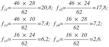
With the chi-square test, prior to the calculation of empirical value, it is necessary to calculate the expected frequencies (fe) in the cells typical for the total absence of relations between variables, and then to compare them with the available frequencies (fo). To do this, the marginal frequency in the column must be multiplied by the marginal frequency in the row and divided by the total number of observations, for each cell:

where MFR is the marginal frequency in the row, MFC is the marginal frequency in the column, N is the total number of observations.
For our example, the calculation of expected frequencies will be as follows:
For our example, the calculation of expected frequencies will be as follows:
Consequently, the table with the theoretical distribution characterized by the total absence of relations between variables will be as follows:
| Efficiency | Gender |
Total
|
|
Female |
Male |
||
| Satisfactory (with D and/or E) | 20,8 |
7,2 |
28 |
| Good or Excellent (no D/E, only B/C/A) | 17,8 |
6,2 |
24 |
| Excellent (only A) | 7,4 |
2,6 |
10 |
| Total | 46 |
16 |
62 |
If the difference between these frequencies and those obtained in the research are great enough, the alternative hypothesis will be adopted by, if not – the null hypothesis will be applied.
Difference value is determined with the help of special index / exponent, which is the empirical (or experimental) test value:
Difference value is determined with the help of special index / exponent, which is the empirical (or experimental) test value:
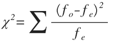
In our case, the empirical test value is equal to:
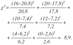
In addition to empirical value, most methods of statistical hypothesis testing involve the calculation of degrees of freedom (df), which are used in determining critical value, i.e. the value empirical value is compared with. This comparison estimates if empirical value is high enough (it must exceed critical value) to reject the null hypothesis and accept the alternative one. For the chi-square test df=(r-1)(c-1), where r is the number of rows in the table, c is the number of columns. Accordingly, in our case df=(3-1)(2-1)=2.
Step 5. All methods of statistical hypothesis testing involve the use of certain sample statistics distributions to determine critical value in each case study. Critical value, as well as empirical, is a special value that sets the limit which, when exceeded, states that there is a very low probability (this probability is equal to the alpha value) that the available results could be obtained due to random errors.
Step 5. All methods of statistical hypothesis testing involve the use of certain sample statistics distributions to determine critical value in each case study. Critical value, as well as empirical, is a special value that sets the limit which, when exceeded, states that there is a very low probability (this probability is equal to the alpha value) that the available results could be obtained due to random errors.
Chi-square distribution used for the analysis of contingency tables changes its form depending on the number of degrees of freedom. Consequently, the distribution of critical values changes as well (df is marked as k in the graph below):
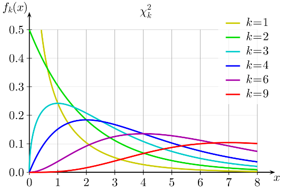
In each specific case, critical value itself is determined with the tables of critical values. With the chi-square test the table has two parameters – the number of degrees of freedom and the alpha level.
After critical value is determined, it must be compared with the empirical value – if critical value is higher, the null hypothesis is adopted (because the probability of obtaining results due to random errors is too high), if empirical value is higher, the alternative hypothesis is adopted.
For our example, the alpha value of 0.05 and df of 2 render the critical value of 5.99. Since the empirical value is higher than the critical value (8.9>5.99) the alternative hypothesis may be adopted. The probability of falsity in this case is 5%.
It is always important to remember that with statistical inference the researcher runs the risk of making a mistake, regardless of what hypothesis he/she adopts – null or alternative. Such errors are called statistical and are divided into two groups – type I and type II errors. With type I errors, the alternative hypothesis is adopted based on the sample data, while the null hypothesis is true for the population. With type II errors, the null hypothesis is adopted based on the sample data, while the alternative hypothesis is true for the population.
- default_titleХили Дж. Статистика. Социологические и маркетинговые исследования. - К.: ООО "ДиаСофтЮП"; СПб.: Питер, 2005. - 638 с.
- default_titleМалхотра Н. Маркетинговые исследования. - М: Вильямс, 2007. - 1200 с.
- default_titleField A. Discovering statistics using SPSS. - London, Thousand Oaks, New Delhi: Sage, 2009. - 822 p.
- Show More