Types of statistical methods: descriptive statistic
Scales of measure >> Descriptive statistic > Analysis of paired association >> Statistical inference
Quantitative data analysis begins with description. Appropriate methods are very simple, but at the same time – very informative.

Dembitskyi S. Types of statistical methods: descriptive statistic [Electronic resource]. - Access mode: http://www.soc-research.info/quantitative_eng/6.html
According to a widely used typology, statistical methods can be divided into descriptive statistics and statistical inference. Descriptive statistics is used for the simple generalization of data obtained under sampling study. In turn, statistical inferences are needed to ensure that the data obtained from the sample can be extended to the entire population.
The basic methods of descriptive statistics include percentages, measures of central tendency, measures of variation and paired relationship coefficients. They allow us to generalize the data obtained for the sample.
The basic methods of descriptive statistics include percentages, measures of central tendency, measures of variation and paired relationship coefficients. They allow us to generalize the data obtained for the sample.
Percentages are used in order to bring the frequency distribution of a variable to 100 (similarly, proportions are used to bring the data to 1). In this form, the data are preferable in the intuitive sense to the "raw" frequency distribution. An example (examinations efficiency):
| Efficiency | Frequency |
% |
Proportions |
| Satisfactory (D/E) | 28 |
45,2 |
0,452 |
| Mostly Good (no D/E, mostly B/C) | 11 |
17,7 |
0,177 |
| Mostly Excellent (no D/E, mostly A) | 13 |
21,0 |
0,210 |
| Excellent (A) | 10 |
16,1 |
0,161 |
| Total | 62 |
100,0 |
1,000 |
Measures of central tendency (mode, median and arithmetic mean) provide information about the typical or central value of distribution. Mode refers to the most frequently occurring value, median – to the medial value, arithmetic mean – to the highest expected value.
The example above, the mode is the option "Satisfactory (D/E)", as it marked by 28 people – more than any other option.
To find the median, we need to organize all the options in their ascending or descending order – first all options "Satisfactory (D/E)", then all options "Mostly Good (no D/E, mostly B/C)", etc. If we have an odd number of observations, we need to find the value that is in the middle of this ranked row. It is this value that is the median. If the number of observations is even, we need to take two values that are in the middle and find their mean. Since in our case there are 62 observations, observation 31 and 32 will be in the middle. This is the "Mostly Good (no D/E, mostly B/C)" option. Consequently, "Mostly Good (no D/E, mostly B/C)" will be the median.
The first chapter illustrates how to calculate the arithmetic mean. In our case, the calculation of the average is not quite correct. However, if we assign specific numeric values to the options (e.g., 1, 2, 3, 4) we can calculate the average.
Measures of variability indicate the degree of heterogeneity of distribution (e.g., range, Index of Qualitative Variation, standard deviation, standard deviation, etc.). Range (R) is the simplest both in terms of the received information and in terms of calculation. It is equal to the difference between the highest and the lowest values of distribution. For example, if the lowest height among respondents is 147 cm and the greatest is 198 cm, the range will be 51 cm.
For quantitative attributes the lowest limit of measures of variability is 0 (observed objects do not differ in the characteristics the researcher is interested in). The upper limit is always an open value defined by the peculiarities of the studied property and the observed heterogeneity of distribution. For example, the standard deviation for the increase in the population of Ukraine in 2008 was 9 cm (the average is 169 cm), and for age it was 17 years (the average is 46 years). Since the calculation of the standard deviation was discussed earlier, here we only touch upon the Index of Qualitative Variation (IQV) – the only measure of variability whose use is entirely correct in case of both nominal and ordinal scales. In this case, the coefficient may range from 0 (no variation) to 1 (maximum variability).
For quantitative attributes the lowest limit of measures of variability is 0 (observed objects do not differ in the characteristics the researcher is interested in). The upper limit is always an open value defined by the peculiarities of the studied property and the observed heterogeneity of distribution. For example, the standard deviation for the increase in the population of Ukraine in 2008 was 9 cm (the average is 169 cm), and for age it was 17 years (the average is 46 years). Since the calculation of the standard deviation was discussed earlier, here we only touch upon the Index of Qualitative Variation (IQV) – the only measure of variability whose use is entirely correct in case of both nominal and ordinal scales. In this case, the coefficient may range from 0 (no variation) to 1 (maximum variability).
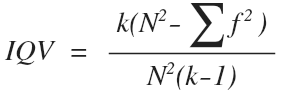
where k is the number of categories of a variable, N is a total number of observations in the sample, Σf^2 is the sum of squares of frequencies.
Let us consider the IQV for the example with students’ efficiency. In order to calculate this coefficient manually it is convenient to use the special table (as well as many other statistics):
| Efficiency | Frequency |
Square of frequency |
| Satisfactory (D/E) | 28 |
784 |
| Mostly good (no D/E, mostly B/C) | 11 |
121 |
| Mostly excellent (no D/E, mostly A) | 13 |
169 |
| Excellent (A) | 10 |
100 |
| Total | N = 62 N^2 = 3844 |
∑f^2 = 1174 |

Paired relationship coefficients serve to analyze the strength and direction of relations between variables. This class encompasses a fairly large number of methods that can be divided into two groups depending on the form of data representation. The first group is used for the analysis of variables that have a small number of categories and are represented in the form of contingency tables (e.g., Cramer’s V for nominal variables and Gamma for ordinal ones).
| Efficiency | Gender |
Total |
|
Female
|
Male |
||
| Satisfactory (with D and/or E) | 16 |
12 |
28 |
| Good or Excellent (no D/E, only B/C/A) | 20 |
4 |
24 |
| Excellent (A) | 10 |
0 |
10 |
| Total | 46 |
16 |
62 |
Contingency tables are intended to provide data on the relationship between two variables. To improve the information content, percentages must be calculated separately for each of the columns. In the example above, the corresponding table is as follows:
| Efficiency | Gender |
Total
|
|
Female |
Male |
||
| Satisfactory (with D and/or E) | 34,8% |
75,0% |
45,2% |
| Good or Excellent (no D/E, only B/C/A) | 43,5% |
25,0% |
38,7% |
| Excellent (A) | 21,7% |
0,0% |
16,1% |
| Total | 100,0% |
100,0% |
100,0% |
The second group of methods is used in the situations where the variables have a large number of categories and there are no clear boundaries for their grouping, or when such grouping may result in the partial loss of information (e.g., Pearson’s or Spearman’s correlation coefficients) [Read more].
Calculation of relationship coefficients is more complex than the methods described earlier. It is better to turn to specialized literature to learn of the relevant formulas and their use. At the level of descriptive statistics, paired relationship can be analyzed in terms of its strength as well as its nature and / or direction.
Relationship strength may range within the interval from 0 to 1 (if at least one variable belongs to the nominal scale: for example, the relation between gender and studying efficiency) or from -1 to +1 (if both variables belong to the ordinal scale: for example, the relation between the level of education and the level of income). Complete absence of relations corresponds to 0, the maximum relationship is observed both at -1 and +1. Maximum relationship strength is a scientific ideal. Consequently, in real life, the values of the corresponding coefficients fall between -1 and 0, or 0 and +1. For example, the relation between height and weight is +0.38 for men, and only +0.18 for women (Ukraine, 2008).
Relationship sign indicates its direction. Negative relationship indicates that with the increase of one variable's value the other variable’s value will decrease. If the relationship is positive, the values of both variables will change in one direction. The relationship between height and weight, thus, is positive. Consequently, taller people are more probable to have greater weight. The example of the negative relationship is the link between the amount of alcohol consumed at night and the way one feels in the morning.
A more detailed relationship analysis is discussed in the next chapter.
- default_titleХили Дж. Статистика. Социологические и маркетинговые исследования. - К.: ООО "ДиаСофтЮП"; СПб.: Питер, 2005. - 638 с.
- Show More